
Why Numerical Solutions?
Mathematically, not every differential solutions is easily solved. In fact, many important physics equation are currently approached using approximation methods. When that is the case, the “frontal attack” approach of direct solutions must be replaced with a more indirect one.
What are Incremental Solutions?
The first equation is the force equation. But we can write this in increments as in the second equation.

What this says is that for an small interval at some time t, we know the change in velocity can be computed using this second formula.
Now suppose we start our small intervals off at time t =0 and keep computing them to our final value of t, we could generate v(t) a set of values without having access to its underlying formula. Sometimes you have to give up some things to get others.
Using Spreadsheets to obtain solutions
You can see how this approach lends itself to a spreadsheet where each interval builds on the previous row of data. You might be bothered using the mid velocity. You might want to use the value at the start or the value at the end. But here is where making Δt small reduces any possible error due to the approximation method.
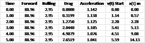
Here is an example for riding on the flats with pedaling producing a forward force of 20 lbs. (Remember this can be much larger at the pedals depending on the gearing). We are assuming a CyclistCycle of 160 lbs riding in the hoods. The forward force and rolling resistance are constant, so the only thing changing is the velocity dependent drag.
The spreadsheet is set up as follows. Each row corresponds to a time starting at 0 seconds and ending at 60 seconds. We assume for each row drag can be approximated using the velocity at the interval start. Then we subtract Rolling and Drag from forward to get the net force. Dividing that by the CyclistCycle mass gives the acceleration over that interval.
Since each interval is 1 second, we get the velocity at the start of the next interval by adding this to the previous velocity. Then we compute the drag using the velocity at the interval start. Using that we compute the acceleration during this next interval.
We compute the velocity by taking the previous velocity at the previous interval start and add its acceleration. Then, to get the position, we add the distance covered for the previous interval start and add to it the velocity at the start and finally half of the acceleration. This last step adjusts for the acceleration increasing throughout the second.
You can now see how this approach yields the numerical results for our motion equations without having to know the underlying formulas.
Next Topic: Comparing Exact and Numerical Solutions